How Sure Is "Sure"? — Calibration, Uncertainty, and Knowledge in LLMs
A hands-on experiment in calibrated confidence: a 150M-parameter student, a 7B teacher's doubts, six training targets, and three kinds of new data. What transfers, what doesn't, and why.
I trained more than 30 small classifiers to learn not just the right answer, but how much to trust it. The first result was a no. Here's what it took to get a yes, and where honesty still isn't enough.
"90% sure" should mean something
If a model says it is 90% confident, then across many predictions made at that confidence level, it should be right about 9 times out of 10.
That sounds obvious, but a lot of real systems depend on it. A support tool that routes tickets automatically when it's confident, and sends the rest to a human. A moderation filter that only acts above a threshold. A pipeline that asks a bigger, more expensive model only when a small one is unsure. All of them treat the model's confidence as a promise.
Most models break that promise. Modern neural networks are often overconfident: they say 95% when they're right 80% of the time. And large language models asked for a single answer can sound certain whether they are or not.
Calibration is not the same as confidence. Confidence is what the model reports. Calibration asks whether those reported probabilities match what actually happens over many predictions.
So I set out to build a small model whose confidence actually means something. The idea: train it on a bigger model's doubts, not just its answers. Instead of telling the student "the answer is billing", tell it "the teacher thought billing 77%, technical 22%, sales 1%", and hope the student learns the shape of the uncertainty along with the answer.
It didn't work the first time. Fixing it taught me more than the success would have.
What calibration means, in one picture
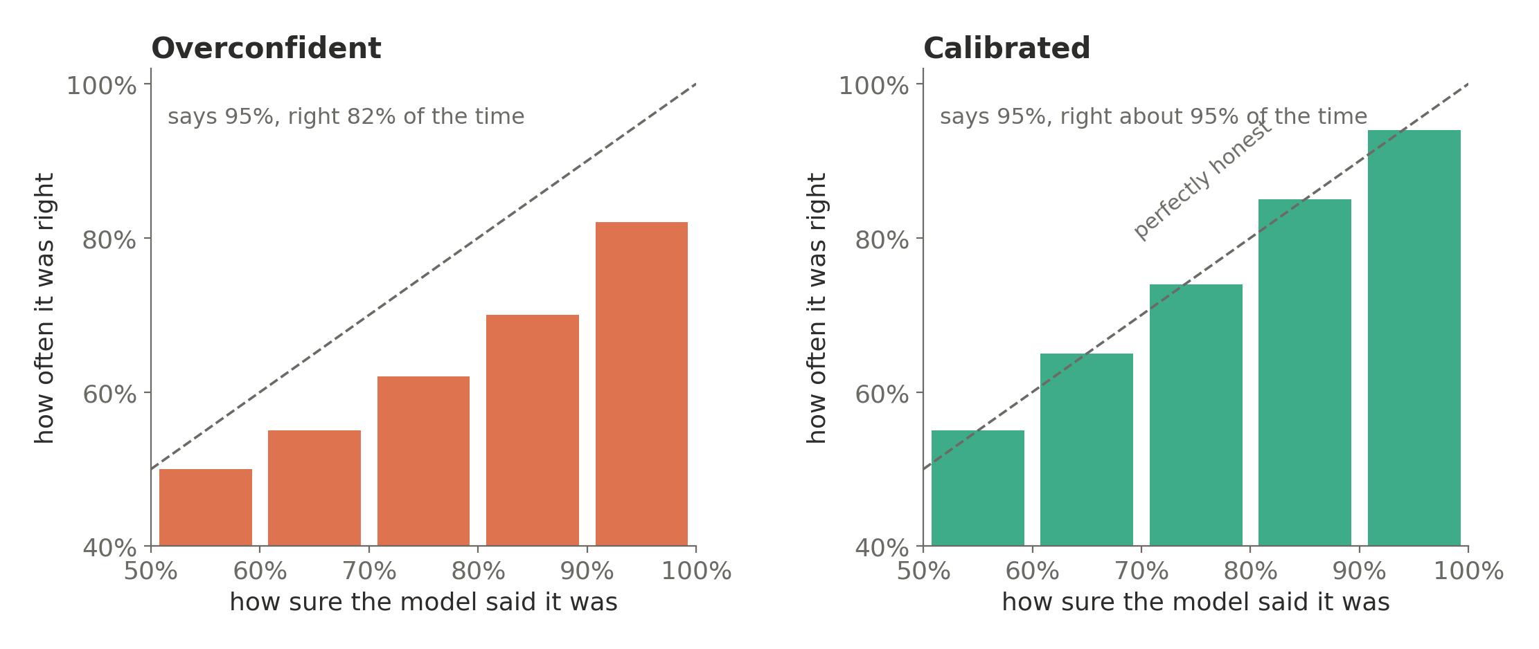
A reliability diagram groups predictions by how confident the model was, then checks how often each group was right. On the dashed line, confidence matches reality.
A useful distinction: uncertainty is what the model believes about its uncertainty; calibration is whether that belief matches reality.
Three numbers summarize this throughout the article:
- Accuracy — how often the model's top pick is the right one. It says nothing about confidence, just hits and misses. An accuracy of
0.907means the model got about 91 questions right out of every 100. - ECE (expected calibration error) — how far the model's stated confidence sits from what actually happens, averaged over all its predictions. An ECE of
0.05means it is off by about 5 percentage points: when it says 90%, it is really right about 85% of the time. An ECE of0.006is near-perfect honesty. Lower is better. Two caveats: ECE measures the size of the gap, not which way it leans, and it depends on how predictions are grouped into bins, so it is best read as a diagnostic rather than an absolute score. - Log loss — one score for the whole set of probabilities, not just the top pick. It rewards putting high probability on the right answer and punishes confident mistakes hardest: being wrong after saying 95% costs far more than being wrong after saying 55%.
0would be perfect, and lower is better. It is the number that notices the difference between a model that is wrong and knew it might be, and one that is wrong and sure.
And one classic fix sets the bar for everything that follows:
A dial. After training, divide all of the model's raw scores by one number before turning them into probabilities. A number above 1 makes every answer less extreme; below 1, more extreme. It's called temperature scaling, it's fitted on a held-out set, and it never changes which answer the model picks, only how sure it sounds.
The dial is cheap and surprisingly strong. Any fancier idea has to beat "train normally, then turn the dial".
The setup
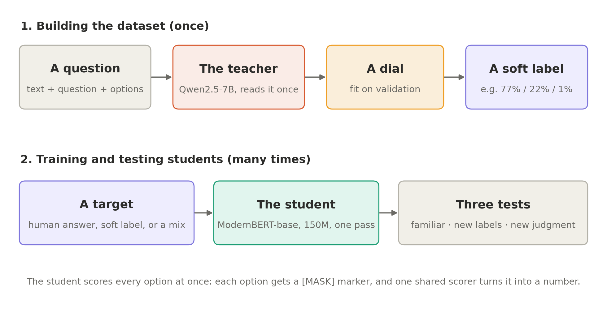
Every example is a typed decision: a piece of text, a question, and a set of options.
Which intent best describes this request?

"How far is it to the nearest charging station?"

A. directions        B. distance        C. traffic        D. travel alert
Some are multiple choice like this one; others are yes/no ("Is this request about: distance?").
The teacher is Qwen2.5-7B-Instruct, run in 4-bit on a free Colab GPU. It reads each question once, and instead of letting it write an answer, I read the probabilities it assigns to each option letter. Those chances are then adjusted by a dial fitted on validation data, and stored as the question's soft label.
A soft label is the teacher's whole opinion rather than its verdict: the "billing 77%, technical 22%, sales 1%" from earlier, instead of a flat "billing". A hard label is the opposite — 100% on one option, 0% on everything else. The whole experiment is a question about which of the two makes a better teacher.
The student is ModernBERT-base, about 150M parameters, roughly 50 times smaller than the teacher. It reads the whole question in one pass, with a [MASK] marker in front of each option. A single shared scorer, 769 numbers in total, turns each marker into a score. Because the scorer is shared, the options can change from one question to the next: the student isn't memorizing a fixed list of labels, it's judging how well each option fits.
The data comes from six public sources, all permissively licensed: three intent datasets (CLINC, Banking77, MASSIVE), emotions in Reddit comments (GoEmotions), product reviews (Amazon Polarity), and why research papers cite each other (SciCite). About 17,000 training questions in total, published as calibrated-typed-decisions.
The hypothesis: a student trained on the teacher's soft labels should end up better calibrated than one trained on plain right answers, especially on data it has never seen.
The first answer was no
The first version of the dataset gave a clear result, just not the one I wanted:
| Accuracy | ECE | Log loss | |
|---|---|---|---|
| Teacher (7B) | 0.875 | 0.019 | 0.385 |
| Student, soft labels | 0.870 | 0.036 | 0.365 |
| Student, right answers | 0.905 | 0.060 | 0.383 |
| Student, right answers + one dial | 0.907 | 0.025 | 0.297 |
Soft labels did make the student more honest than plain right answers (ECE 0.036 vs 0.060). But one dial, fitted after training, erased that advantage: the plain student with a dial came out the most accurate and with the best log loss of all, beating its own teacher. (The soft-label student with its own dial reached an ECE of 0.027: no better.) The fancy method lost to the simple baseline.
The reason became clear on one source. GoEmotions is genuinely hard (is a comment "annoyance" or "disapproval"?), and the teacher was right only 60% of the time on it:
| GoEmotions, choice questions | Accuracy |
|---|---|
| Teacher | 0.602 |
| Student trained on the teacher's soft labels | 0.653 |
| Student trained on human answers | 0.810 |
A student can't be much more right than the labels it learns from. Soft labels carry the teacher's doubts, but they also carry its mistakes, with high weight. Where the teacher was weak, the soft-label student inherited the weakness.
That changed the question. Not "do soft labels work?", but "what would soft labels need to be worth using?"
Fixing the data, not the model
The second version of the dataset kept the student and the training code exactly the same, and changed the data:
- Human votes instead of the teacher, where they exist. GoEmotions comes with the individual votes of several human raters. On 600 questions, the teacher's top pick disagreed with the official answer
38.5%of the time; the raters' top pick matched it96.7%of the time. So for GoEmotions, the soft label became the raters' vote shares. - Descriptions for every option, so "qa stock" becomes "qa stock: asking about the price of a stock".
- Harder wrong options. Instead of random distractors, the wrong options are the labels closest in meaning to the right one, so the student has to actually read.
- A sixth source, SciCite, and more questions per source.
- A held-out test from a different world. 1,000 expert-labelled PubMedQA questions: a medical research question, an abstract, and "does the evidence support yes, no, or maybe?" No student ever trains on it.
The GoEmotions fix alone moved the soft-label student on that source from 65% to 88% accuracy, now above the student trained on human answers. (Different test questions between versions, so not a perfect comparison, but the reversal is unmistakable.)
One more fix came later, in version 2.1. On about 1 in 10 teacher-labelled training questions, the teacher's top pick was wrong. A new column, corrected_soft_label, keeps the teacher's numbers but swaps them so the right answer always gets the largest share. The teacher's opinion about which wrong answer is the most confusable survives; its mistake doesn't.
Six students, one variable
With the data fixed, I trained six students. Everything is identical (model, data, steps, learning rate) except the target each one learns from:
| Run | What the student learns from |
|---|---|
| A | the human answer only (100% on one option) |
| B | the human answer, softened evenly (a small share spread over the others) |
| C | the teacher's soft label |
| D | half A, half C |
| E | the corrected teacher (corrected_soft_label) |
| F | half A, half E |
Here's what they look like on one real training question, where the right answer is "distance" and the teacher favoured "directions":
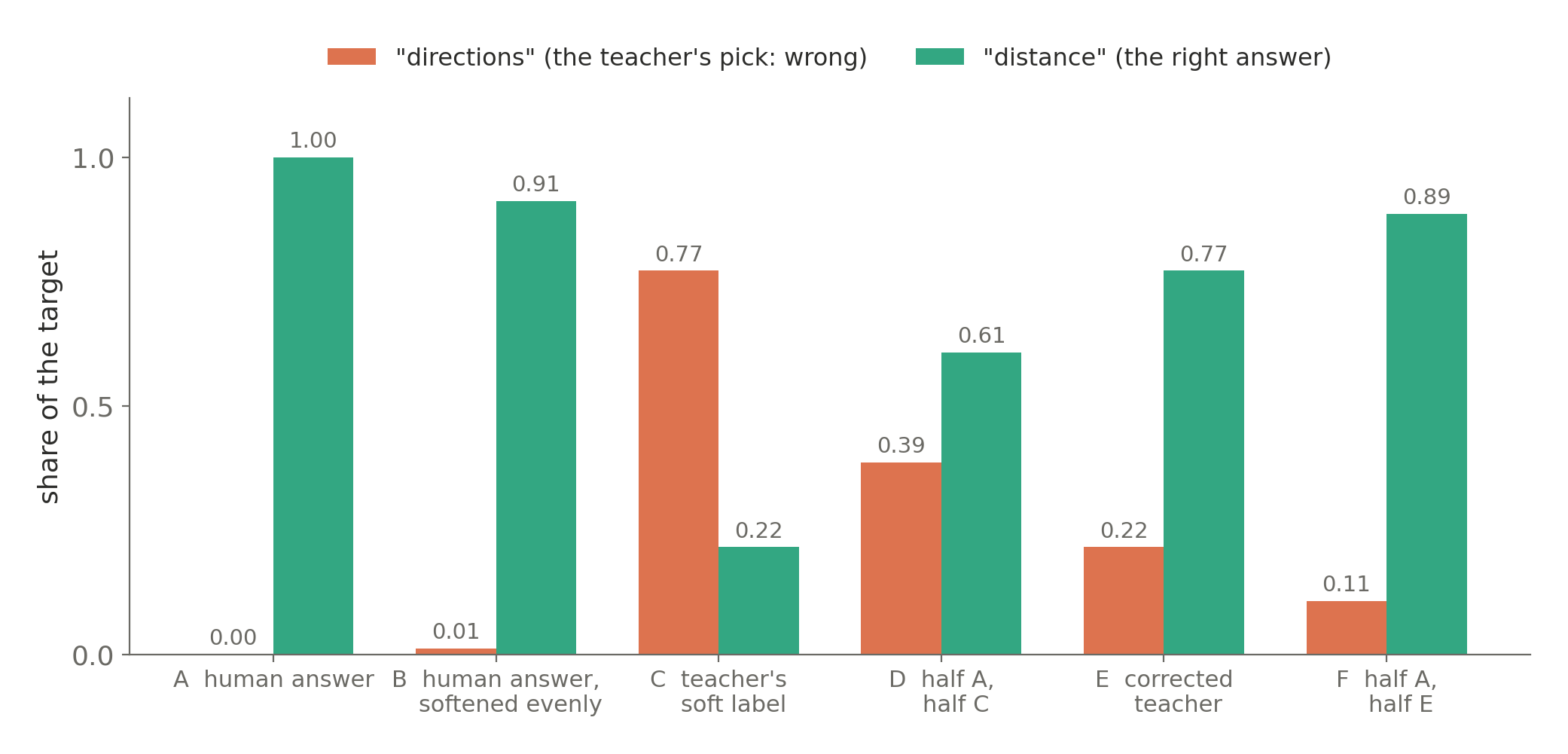
C learns the teacher's mistake. D halves it. E fixes it but keeps the teacher's sense that "directions" is the closest wrong answer. F does the same with more weight on the right answer.
The recipe, identical for every run:
| Student | ModernBERT-base (~150M) + one shared scorer (769 numbers) |
| Training | 3 epochs, batch 16, AdamW (weight decay 0.01), 10% warmup, gradient clipping at 1.0, mixed precision |
| Learning rates | 3e-5 for the pre-trained body, 1e-3 for the new scorer |
| Kept epoch | the one with the lowest validation log loss |
| After training | 2 dials fitted on validation (one for choice, one plus a yes/no shift for yes/no) |
| Repeats | 3 seeds per run, averaged into an ensemble |
| Cost | about 20 minutes per run on a free Colab T4 |
Being suspicious of my own results
This is the part I didn't plan for, and the part that mattered most. Three times, a result that looked like a finding turned out to be partly luck.
1. One dial, or twelve? My first version fitted a separate dial for each source and question type: twelve in total. That turned out to be too many: with only a couple of hundred validation questions behind each one, the dials started fitting noise. For one student, twelve dials gave a worse result than no dial at all. Comparing the options fairly, by fitting dials on one half of the validation set and scoring on the other, two dials (one for multiple choice, one for yes/no) won for every student:
| Dial setup | Validation log loss (lower is better) |
|---|---|
| no dial | 0.262 |
| 12 dials | 0.252 |
| 2 dials | 0.242 |
2. One training run lies. A seed is the random number that fixes where the new weights start and the order the examples arrive in. Same model, same data, same settings — change only the seed and you get a different model. Training the same recipe again with a different random seed changes the result. On my first single run, the 50/50 blend (D) looked like the clear winner on familiar data. After two more seeds, the win dissolved: the first seed happened to be D's luckiest and A's unluckiest. On the medical held-out test, retraining alone moved student A's accuracy from 0.538 to 0.614. A single run can't tell you which target is better.
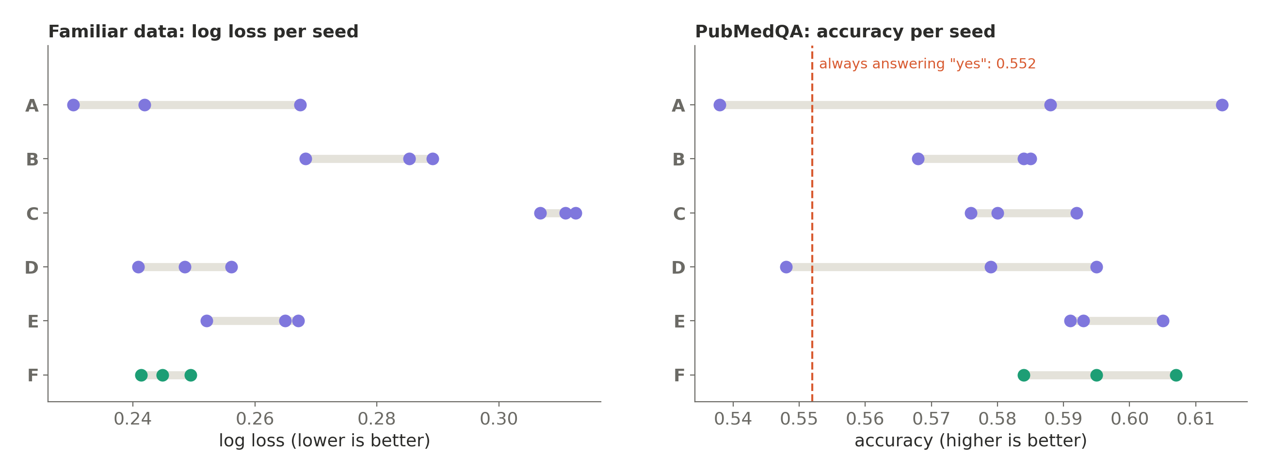
Each dot is one training run. At home, luck is small. On unfamiliar data, it's large enough to flip a conclusion.
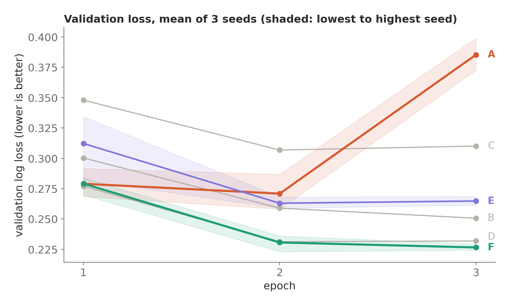
The training curves add one more hint. The student trained on hard answers (A) is the only one whose validation loss jumps in the third epoch, from 0.271 to 0.385 on average, while every other run levels off or keeps improving. Hard targets keep pushing a student to be more certain, and past a point that certainty stops being earned. (Each run keeps its best epoch, so this doesn't hurt A's final results, but it shows the pull.)
3. A rule I wrote down before looking. From then on, every student was trained three times, the three were averaged into an ensemble, and a comparison counted as real only if it held in every seed and in a bootstrap over the test questions for the ensembles.
An ensemble here means averaging the three runs' predicted probabilities into a single prediction — 3 models in, 1 answer out. The point is that it is an average, not a pick: choosing whichever seed scored best would be grading my own luck. A bootstrap re-scores that same test set many times over random resamples of its questions, which shows whether a gap between two students survives, or whether it was an accident of which questions happened to land in the test.
Before training F, I wrote down that F would count as better than D only if it passed both checks. It didn't, quite: the average gap favoured F in five of six comparisons, but none of them held in every seed and in the ensemble check. So the honest verdict is "probably a little better, not proven".
Three kinds of new
Testing only on data like the training set tells you very little about honesty. The real question is what happens when something is new. So every student faced three tests:
- Familiar: test questions from the six training sources.
- A new label set: SNIPS, 1,050 voice-assistant requests with 7 intents the students had never seen (none of its requests appear word-for-word in the training data).
- A new kind of judgment: PubMedQA, where the task isn't "which category is this?" but "does this evidence support the claim?"
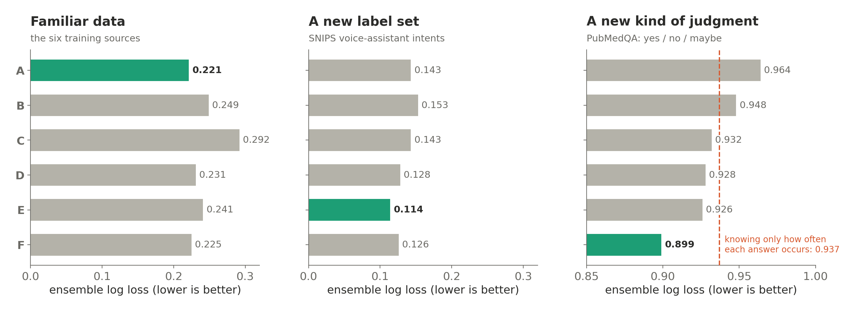
Here's every run's ensemble on all three:
Familiar data: the simple baseline holds up
On data like the training set, the hard-label student with a dial (A) and the corrected blend (F) are statistically tied: ensemble log loss 0.221 vs 0.225. F's ensemble is the most accurate (0.928) and the most honest (ECE 0.006), but the difference from A is within luck. The teacher's raw soft labels (C) are reliably the weakest, for the reason v1 showed.
All students beat their teacher here, by a lot: about 89–92% accuracy against the teacher's 84%.
A new label set: almost no drop, and E leads
On SNIPS, the students score about as well as on MASSIVE, a dataset of the same kind they did train on. Accuracy, single students, mean of 3 seeds:
| A | B | C | D | E | F | |
|---|---|---|---|---|---|---|
| MASSIVE (seen) | 0.948 | 0.951 | 0.921 | 0.955 | 0.949 | 0.954 |
| SNIPS (never seen) | 0.949 | 0.948 | 0.951 | 0.953 | 0.960 | 0.950 |
A student trained to pick intents can pick intents from a label set it has never seen. C even does better on SNIPS than on MASSIVE: on MASSIVE it inherits the teacher's mistakes between close labels, and SNIPS's seven intents are easy to tell apart.
(SNIPS has only 7, fairly distinct intents, so its questions are probably easier than MASSIVE's. "No drop" partly reflects that. Still, near-perfect accuracy on brand-new labels is real evidence of a general skill.)
And here, the fully teacher-shaped target wins: E's ensemble has the lowest log loss (0.114, accuracy 0.965), and beat A, B, and F under both checks. It's honest there too, with an ECE of 0.020 (the middle row of the reliability figure below). On familiar data, mixing in the hard answer (F) helps; on a new label set, keeping the teacher's softer shape (E) transfers better.
A new kind of judgment: honest, but not knowledgeable
PubMedQA is where everything gets humbling. A predictor that ignores the abstract and only knows how often each answer occurs scores a log loss of 0.937. Always answering "yes" scores 55.2% accuracy.
The best student, F's ensemble, scores 0.899 and 59.5%. That's the first student to clear the "know nothing" line properly, but only just.
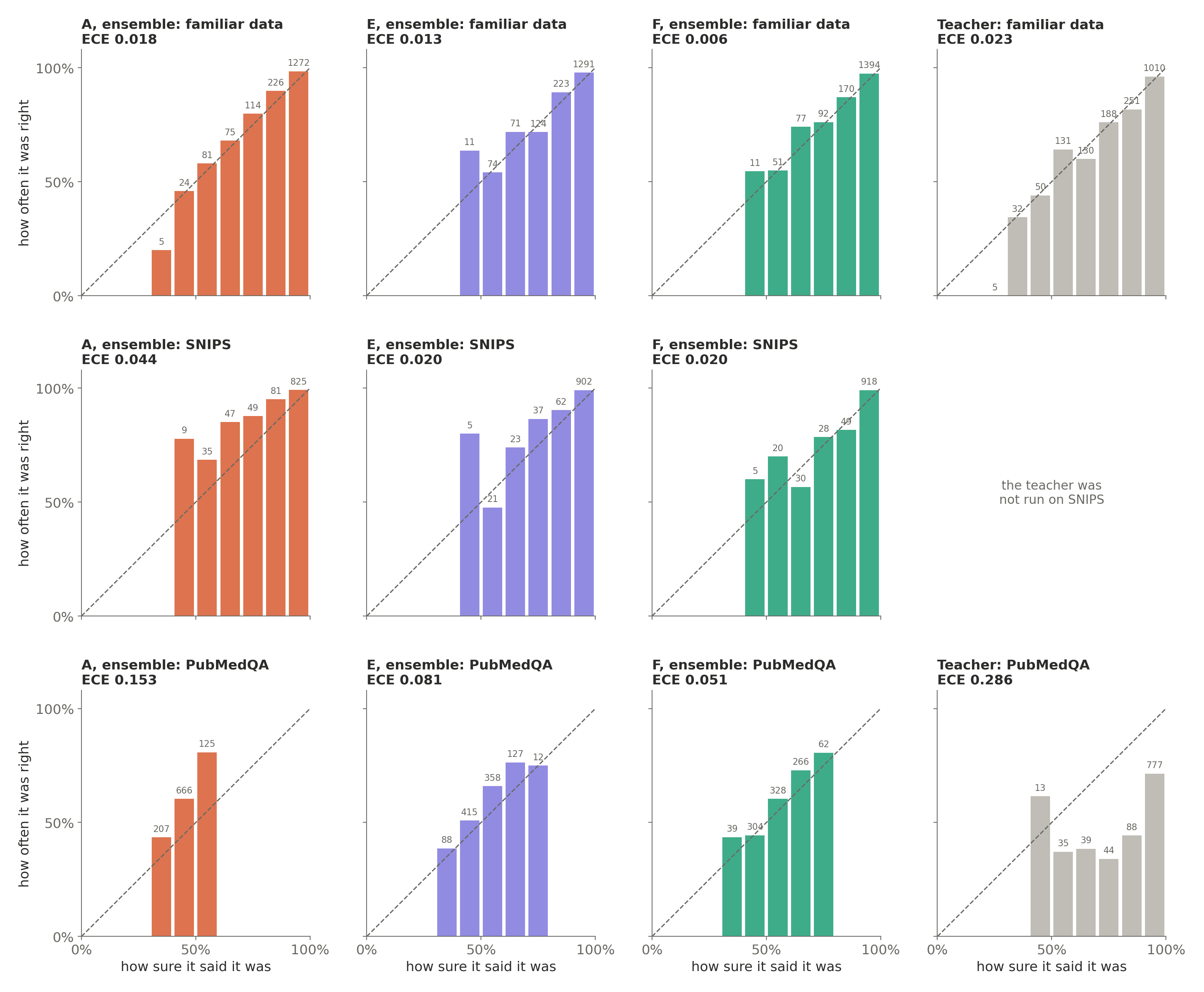
The reliability diagrams show what did transfer, and one thing I didn't expect.
A is badly miscalibrated on PubMedQA (ECE 0.153), but underconfident, not overconfident. It never says more than 60%, yet in its 50–60% group it's right 81% of the time. The likely reason: its dials were fitted on familiar data, where a hard-label student needs strong toning down, and carried over to PubMedQA, the same dials flatten it too much. Without its dials, A's PubMedQA log loss would actually be better (0.924 instead of 0.964). The same effect shows up, more mildly, on SNIPS, where A's bars also sit above the line (ECE 0.044, against 0.020 for E and F). A dial fitted on one kind of data doesn't automatically travel.
F stays close to the line (ECE 0.051). C, D and F were all reliably more honest than A on PubMedQA, under both checks.
The teacher is the overconfident one. For all its 7 billion parameters, 777 of its 1,000 PubMedQA answers came with 90%+ confidence, and only about 71% of those were right. Overall it's 64.7% accurate, with an ECE of 0.286 and a log loss of 2.33: confidently wrong often enough to be dangerous.
So the soft labels did teach something real: how to be unsure on unfamiliar data. What they couldn't teach is how to judge biomedical evidence, because nothing in the six training sources ever asks for that.
Why averaging didn't save it
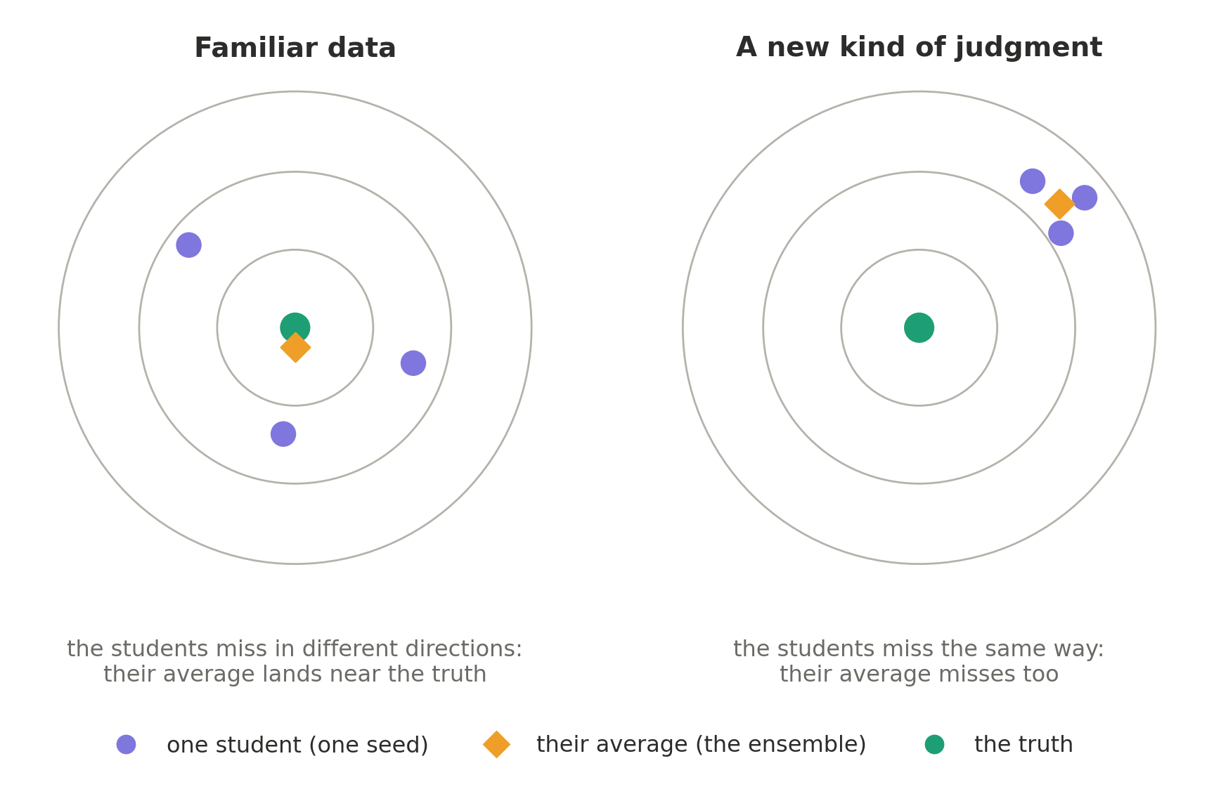
Ensembles helped a lot on familiar data: every run's average of three beat even its best single seed (for A, log loss went from 0.247 for a typical single student to 0.221 for the ensemble). On PubMedQA they barely helped (0.970 to 0.964). Averaging cancels disagreement between students (variance), but not a mistake they all share (bias). The students all lacked the same skill, so their average lacked it too.
That's the clearest way I can put the result: calibration is about meaning what you say. Knowledge is about having something useful to say.
A model can learn to express uncertainty without learning the underlying skill. A weather forecaster who says "30% rain" every day, in a city where it rains 30% of days, is perfectly calibrated and completely useless. On PubMedQA, my students are close to that corner. No dial fixes it; only more knowledge does.
What I actually learned
- Calibration and confidence are not the same thing. A model can sound uncertain without being well calibrated, and a calibrated model is one whose probabilities have meaning over many predictions.
- The dial is a brutally strong baseline. "Train on right answers, then fit one temperature" beat my first soft-label attempt outright, and it's still tied for best on familiar data.
- Soft labels inherit their teacher's ceiling. Their value depends on the teacher being right. Fixing the labels (human votes, corrected top picks) mattered more than any training trick.
- No single target wins everywhere. More weight on the right answer helps on familiar data; more of the teacher's shape helps on new label sets. Pick by where the model will be used.
- One seed lies. Retraining alone moved results by up to 7.6 accuracy points. Every claim in the dataset card now has to hold in every seed and in a bootstrap.
- A dial fitted on one kind of data doesn't automatically travel. The same dials that made A honest on familiar data made it underconfident on PubMedQA.
- Calibrated is not the same as knowledgeable. My students are honest where they have the skill and fairly honest where they don't, but honesty can't replace the skill.
- Measure the data before building with it. Three of four candidate datasets failed checks that took minutes to run.
What's next
The open problem is skill, not calibration.
Calibration can tell you whether a model knows when it might be wrong. It cannot give the model knowledge it never learned.
Two levers are left:
- A bigger student. ModernBERT-large has about 2.6× the parameters and more general reading ability from pre-training. With LoRA, it fits on a free GPU.
- The right training data. A dataset that teaches "does this support that?" without being biomedical, so a PubMedQA gain would show the skill transferred. WANLI is the best candidate, if its license question can be resolved.
The receipts: v1, right answers + one dial: accuracy
0.907, log loss0.297, best of the first round · GoEmotions teacher disagreed with humans on38.5%of questions · 2 dials beat 12 (0.242vs0.252) · retraining alone moved held-out accuracy by7.6points · familiar data: A0.221≈ F0.225· new label set: E best,0.114· new kind of judgment: F best,0.899against a0.937know-nothing baseline · F's ensemble ECE:0.006familiar,0.020SNIPS,0.051PubMedQA · the 7B teacher on PubMedQA:777of 1,000 answers at 90%+ confidence, right about 71% of the time.
Data: CLINC150, Banking77, MASSIVE, GoEmotions, Amazon Polarity and SciCite (training); PubMedQA (held-out) and SNIPS (evaluation only). Licenses and citations for each are on the dataset card.
Built with PyTorch, transformers, and datasets on Google Colab's free tier. The dataset, with every result table and caveat on its card, is on Hugging Face: m-lagnajit/calibrated-typed-decisions. The notebooks are on GitHub.
lagnajit moharana.